Multiple systems estimation
Introduction
It’s often necessary to make population inferences when all we have are multiple, incomplete datasets regarding the population. For instance, we could use a cellphone app to collect reports of bird-sightings from citizen scientists, but then we need to get from bird sightings by cell-phone owners to actual bird populations. Or, we might have reports of human rights violations from multiple sources. In such cases, we know that not all of the population of interest is represented in the data, and furthermore that the data we do have may be systematically biased (reported bird sightings will track where humans with cell phones are when they see a bird, but that may not represent where most birds are; certain types of victims or abuses may be better- or less-well documented than others).
Simulating data
# requirements
library(tidyverse)
library(brms)
library(tidybayes)

theme_set(
    hrbrthemes::theme_ipsum_rc(grid = FALSE) +
        theme(plot.background = element_rect(
            fill = "#fdfdfd", colour = NA
        )))
I’ll use simulation to explore the problem. We have, on the one hand, a
series of events that are uniquely identifiable. However, as analysts,
we won’t have access to a full census of the events – instead we’ll
have access to one or more reporting sources who provide reports of some
subset of all events. We’re interested in both inferring the total
number of events from the incomplete reports, and in understanding the
relative proportions of events of different classes. In other words, we
have to make some inferences about how many events went unreported, and
possibly correct for bias in the reporting sources. By sampling the
unique event_id in the simulation, we’re assuming that we can
de-duplicate the event reports from multiple sources – getting data
into such a state is itself a challenging
problem.
generate_events <- function(
    n = 5000,
    classes = "a",
    class_weights = NULL) {

    class_weights <- standardize_weights(classes, class_weights)

    data_frame(
        event_id    = seq_len(n),
        event_class = sample(names(class_weights),
                             size = n,
                             replace = TRUE,
                             prob = class_weights)
    )
}

## helper function
standardize_weights <- function(classes, class_weights) {
    n_classes <- length(classes)

    if (is.null(class_weights))
        class_weights <- set_names(rep(1, n_classes), classes)

    not_specified <- setdiff(classes, names(class_weights))
    n_not_specified <- length(not_specified)

    if (n_not_specified > 0) {
        extra_wts <- set_names(rep(1, n_not_specified),
                               not_specified)
        class_weights <- c(class_weights, extra_wts)
    }

    class_weights / sum(class_weights)
}
For example, we can simulate two classes of events where one class is 3 times as prevalent as the other:
generate_events(classes = c("a", "b"),
                class_weights = c(a = 3)) %>%
    group_by(event_class) %>%
    summarise(n = n_distinct(event_id))
## # A tibble: 2 x 2
##   event_class     n
##   <chr>       <int>
## 1 a            3799
## 2 b            1201
A reporting source is simulated by sampling from the population of events, possibly with bias. To generate multiple reports of events, we use multiple samples:
sample_events <- function(events, frac = .1,
                          weights = NULL) {

    classes <- unique(events$event_class)
    n_classes <- length(classes)
    weights <- standardize_weights(classes, weights)
    prob <- weights * n_classes

    ev <- split(events, events$event_class)
    map2_df(.x = prob, .y = names(prob),
            ~sample_frac(ev[[.y]], size = .x * frac))
}

generate_reports <- function(events, n_reports = 1, ..., from = 1) {
    res <- rerun(n_reports, sample_events(events, ...))
    imap_dfr(res, ~mutate(.x, source = paste0("source", from + .y - 1)))
}
A simple example: random samples
We start with a simple example. There is only one class of event, and we have no concerns about reports being systematically biased by event class. We know that the reports are incomplete, and we want to estimate the true number of events in the population – this involves estimating how many events went unreported in all of our sources. We have 4 independent sources.
set.seed(93730938)
events <- generate_events(n = 5000)
event_reports <- generate_reports(events, n_reports = 4, frac = .15)
Since we have access to the data generating process, we know the true number of events is 5,000. However, a naive summary of the available data would suggest something much smaller:
event_reports %>%
    summarise(n = n_distinct(event_id))
## # A tibble: 1 x 1
##       n
##   <int>
## 1  2393
The problem we have is analagous to estimating the number of fish in a lake (or jelly beans in a jar) by tagging and releasing a sample and then counting how many tagged specimens appear in subsequent samples. That is, we examine not only how many events were reported by individual sources, but also the number of events reported by multiple sources. If there are a lot of overlapping reports, we conclude that our sources have covered a large fraction of the total events and there aren’t many unreported ones. If, on the other hand, there are few overlapping reports, then we conclude that they are samples from a much larger space, and that there must be many events that went unreported in all sources.
summarize_reports <- function(event_reports) {
    event_reports %>%
        mutate(placeholder = 1L) %>%
        spread(source, placeholder, fill = 0L) %>%
        group_by_at(vars(-event_id)) %>%
        summarise(n = n_distinct(event_id)) %>%
        ungroup
}

event_report_smry <-  summarize_reports(event_reports)

event_report_smry
## # A tibble: 15 x 6
##    event_class source1 source2 source3 source4     n
##    <chr>         <int>   <int>   <int>   <int> <int>
##  1 a                 0       0       0       1   469
##  2 a                 0       0       1       0   456
##  3 a                 0       0       1       1    86
##  4 a                 0       1       0       0   455
##  5 a                 0       1       0       1    79
##  6 a                 0       1       1       0    79
##  7 a                 0       1       1       1    19
##  8 a                 1       0       0       0   473
##  9 a                 1       0       0       1    68
## 10 a                 1       0       1       0    76
## 11 a                 1       0       1       1    15
## 12 a                 1       1       0       0    86
## 13 a                 1       1       0       1    13
## 14 a                 1       1       1       0    18
## 15 a                 1       1       1       1     1
We’ll use the table of counts of events by which sources they were
reported in for our model. What we want to find out is the missing row
in the table – the number of events that were reported in none of the
sources. The trick we can use is to the model event count n (using
poisson regression) in terms of the binary variables encoding presence
in each reporting source. The intercept of the associated linear
model
then tells us the number of events when the indicator variable for every
source is equal to 0. (Since there is only one event class, I’m ignoring
that for now).
event_data_model <- brm(n ~ source1 + source2 + source3 + source4,
                        data = event_report_smry,
                        family = poisson(link = "log"),
                        cores = 4)
## Compiling the C++ model

## Start sampling
event_data_model
##  Family: poisson
##   Links: mu = log
## Formula: n ~ source1 + source2 + source3 + source4
##    Data: event_report_smry (Number of observations: 15)
## Samples: 4 chains, each with iter = 2000; warmup = 1000; thin = 1;
##          total post-warmup samples = 4000
##
## Population-Level Effects:
##           Estimate Est.Error l-95% CI u-95% CI Eff.Sample Rhat
## Intercept     7.87      0.05     7.77     7.98       1488 1.00
## source1      -1.74      0.05    -1.84    -1.64       1663 1.00
## source2      -1.74      0.05    -1.84    -1.64       1827 1.00
## source3      -1.74      0.05    -1.85    -1.64       1860 1.00
## source4      -1.74      0.05    -1.85    -1.64       1890 1.00
##
## Samples were drawn using sampling(NUTS). For each parameter, Eff.Sample
## is a crude measure of effective sample size, and Rhat is the potential
## scale reduction factor on split chains (at convergence, Rhat = 1).
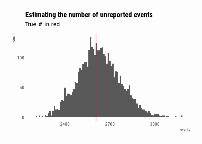
To make inferences about the number of unreported events, I can just sample from the Intercept parameter of the model. Since I used a log-link function, I exponentiate to get back to meaningful units. Since in this case I do happen to know the true number of unreported events, I can compare:
posterior <- posterior_samples(event_data_model, pars = "Intercept") %>%
    mutate(events = exp(b_Intercept))

unreported_events <- length(setdiff(events$event_id, event_reports$event_id))

ggplot(posterior, aes(x = events)) +
    geom_histogram(binwidth = 10) +
    geom_vline(xintercept = unreported_events, colour = "red") +
    labs(title    = "Estimating the number of unreported events",
         subtitle = "True # in red")
Biased sources
As discussed in the introduction, in real life it is generally the case that our reporting sources are not unbiased. If we have a situation where events can belong to different event classes, and the reports over- or under-represent certain classes, can we still make defensible inferences about the underlying population? For this example, we’ll simulate events that can take one of 5 different classes, but our data will include two sources that over-represent certain classes.
set.seed(307037)
complex_events <- generate_events(n = 15000, classes = letters[1:5])

complex_event_reports <-
    bind_rows(
        generate_reports(events = complex_events,
                         n_reports = 4, frac = .1, from = 1),
        generate_reports(events = complex_events,
                         n_reports = 2, frac = .2,
                         weights = c(a = 8, c = 5), from = 5)
    )
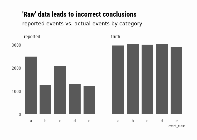
A naive analysis of this data might conclude that, even if we don’t know the exact number of events since our reports are incomplete, we can say that events “a” and “c” are more prevalent. In fact, we would only be describing the bias of our reporting sources:
complex_event_reports %>%
    bind_rows(complex_events %>% mutate(source = "truth")) %>%
    mutate(source = ifelse(str_detect(source, "source"),
                           "reported", "truth")) %>%
    group_by(source, event_class) %>%
    summarise(n = n_distinct(event_id)) %>%
    ggplot(aes(x = event_class, y = n)) +
    geom_col(width = .8) +
    facet_wrap(~source) +
    labs(title    = "'Raw' data leads to incorrect conclusions",
         subtitle = "reported events vs. actual events by category") +
    theme(axis.title.y = element_blank())
We’ll set up the data for the model as before:
complex_event_report_smry <- summarize_reports(complex_event_reports)
complex_event_report_smry
## # A tibble: 211 x 8
##    event_class source1 source2 source3 source4 source5 source6     n
##    <chr>         <int>   <int>   <int>   <int>   <int>   <int> <int>
##  1 a                 0       0       0       0       0       1   498
##  2 a                 0       0       0       0       1       0   476
##  3 a                 0       0       0       0       1       1   500
##  4 a                 0       0       0       1       0       0    54
##  5 a                 0       0       0       1       0       1    50
##  6 a                 0       0       0       1       1       0    57
##  7 a                 0       0       0       1       1       1    54
##  8 a                 0       0       1       0       0       0    51
##  9 a                 0       0       1       0       0       1    48
## 10 a                 0       0       1       0       1       0    63
## # ... with 201 more rows
I can imagine the same sort of model as we used in the simpler case above. If a particular class of event appears in more intersections than another, I can infer that it is over-represented in the data.
complex_event_data_model <-
    brm(n ~ (1 + source1 + source2 + source3 +
                 source4 + source5 + source6) | p | event_class,
        data = complex_event_report_smry, family = poisson(),
        control = list(adapt_delta = .95, max_treedepth = 15),
        iter = 3000, chains = 4,
        cores = 4)
## Compiling the C++ model

## Start sampling

## Warning: There were 37 divergent transitions after warmup. Increasing adapt_delta above 0.95 may help. See
## http://mc-stan.org/misc/warnings.html#divergent-transitions-after-warmup

## Warning: Examine the pairs() plot to diagnose sampling problems
Once again, I can use the intercept of the linear model to estimate the
number of unreported events. This time around, I’ve modeled a global
intercept (called b_Intercept) as well as offsets from the global
intercept for each class. After adding them together, I exponentiate as
before to return to the events-scale. tidybayes::spread_draws allows
me to sample the parameters I’m interested in:
ce_estimates <- complex_event_data_model %>%
    spread_draws(r_event_class[class, param], b_Intercept) %>%
    filter(param == "Intercept") %>%
    mutate(unreported_est = exp(r_event_class + b_Intercept)) %>%
    ungroup

ce_estimates
## # A tibble: 30,000 x 8
##    .chain .iteration .draw class param r_event_class b_Intercept
##     <int>      <int> <int> <chr> <chr>         <dbl>       <dbl>
##  1      1          1     1 a     Inte…       -2.02          8.28
##  2      1          1     1 b     Inte…       -1.05          8.28
##  3      1          1     1 c     Inte…       -1.45          8.28
##  4      1          1     1 d     Inte…       -0.795         8.28
##  5      1          1     1 e     Inte…       -0.909         8.28
##  6      1          2     2 a     Inte…       -1.37          7.54
##  7      1          2     2 b     Inte…       -0.0782        7.54
##  8      1          2     2 c     Inte…       -0.659         7.54
##  9      1          2     2 d     Inte…       -0.0439        7.54
## 10      1          2     2 e     Inte…       -0.252         7.54
## # ... with 29,990 more rows, and 1 more variable: unreported_est <dbl>
I’ll also add back in the reported numbers in order to output an
estimate of the total number of events by class. Finally, plot these
estimates against the true population data from complex_events:
reported_by_class <- complex_event_reports %>%
    group_by(class = event_class) %>%
    summarise(n_reported = n_distinct(event_id))

actual_by_class <- complex_events %>%
    group_by(class = event_class) %>%
    summarise(n = n_distinct(event_id))

ce_estimates %>%
    inner_join(reported_by_class, by = "class") %>%
    mutate(estimated = n_reported + unreported_est) %>%
    ggplot(aes(x = estimated)) +
    geom_histogram(binwidth = 3) +
    facet_wrap(~class, scales = "free_y") +
    geom_vline(data = actual_by_class, aes(xintercept = n),
               colour = "red", size = 1) +
    theme(axis.title.x = element_blank(),
          axis.title.y = element_blank()) +
    labs(title    = "Estimated events by type",
         subtitle = "true # of events in red")

System dependence
This post did not explore the phenomenon of “system dependence” – when an event’s appearance on one list makes it more or less likely to appear on another list. For instance, according to this overview by Lum, Price, and Banks, in the context of documenting human rights abuses,
This was a major problem in the Colombia case study highlighted in Section 3.3, where Benetech analyzed lists collected by both government agencies and nongovernmental organizations (NGOs). Negative dependence occurred because people who were inclined to report a violation to an NGO were less likely to trust the government (and vice versa). Positive dependence occurred because records of homicides kept by the National Police were partially subsumed in the list of violations collected by the Office of the Vice Presidency, and both lists were among those used in the analysis.
The approaches presented in that paper involve adding interaction terms to the model – in fact, looking at every possible model based on presence or absence of each interaction and then either picking the best model or averaging over them.
Resources
Much of what was presented here is based on my understanding of the thorough 5-part FAQ over at the HRDAG website, Patrick Ball’s blog post about the topic, and the paper by Lum, Price, and Banks (paywalled).